by Loic Tudela

Potential future exposure (PFE) is a common risk measure used by sell-side banks to manage counterparty credit risk. PFE measures the tail (near worst case) exposure to the counterparty at a future time point. Banks set limits to this tail exposure to cap the risk they face when a counterparty defaults.

Modelling portfolio exposure

Simplistic approaches approximate PFE by using conservative scaling factors applied to the current value of the trade. While simple to calculate, they do not take into account portfolio concentration risk or other factors that drive future exposure. Sophisticated approaches rely on Monte Carlo simulation of the risk factors that drive portfolio value to generate future distributions of exposure. The PFE at the future time horizon is computed as the 95th percentile of that distribution. Such simulation-based approaches accurately model concentration and diversification risks, as well as the correlation risks that lie within the risk factors that drive the bank's exposure.

The key component of accurately modelling exposures with Monte Carlo simulation is in choosing what risk factors drive the portfolio exposure and determining how they evolve over time. Sell-side bank portfolios are often heavy with swaps and cross-currency swaps, so interest rates and exchanges rates are the main risk factors that will be considered in these stochastic simulations. Should the portfolio also include volatility-sensitive products like vanilla options or more structured exotic products, implied volatility may become an important risk factor.

The simplest and more common choice of dynamics for implied volatility in PFE models is to assume the volatilities are static over the lifetime of the portfolio. However, one need only look at recent market conditions to see that as a crude approximation (see Figure 1). Recent market shocks from global pandemics to geopolitical risks and inflation consistently cause volatility in the implied volatility of assets. For example, the tax cuts proposed in the recent UK budget have driven the implied volatility of the GBP¬-USD exchange rate to highs not seen since the COVID-19 crisis.[1] It therefore seems apparent that any measure of future portfolio exposure should accurately model the future volatility of volatility. We look at the impact on PFE of typical portfolios when the volatility of volatility is included in the stochastic models driving exposure simulations.

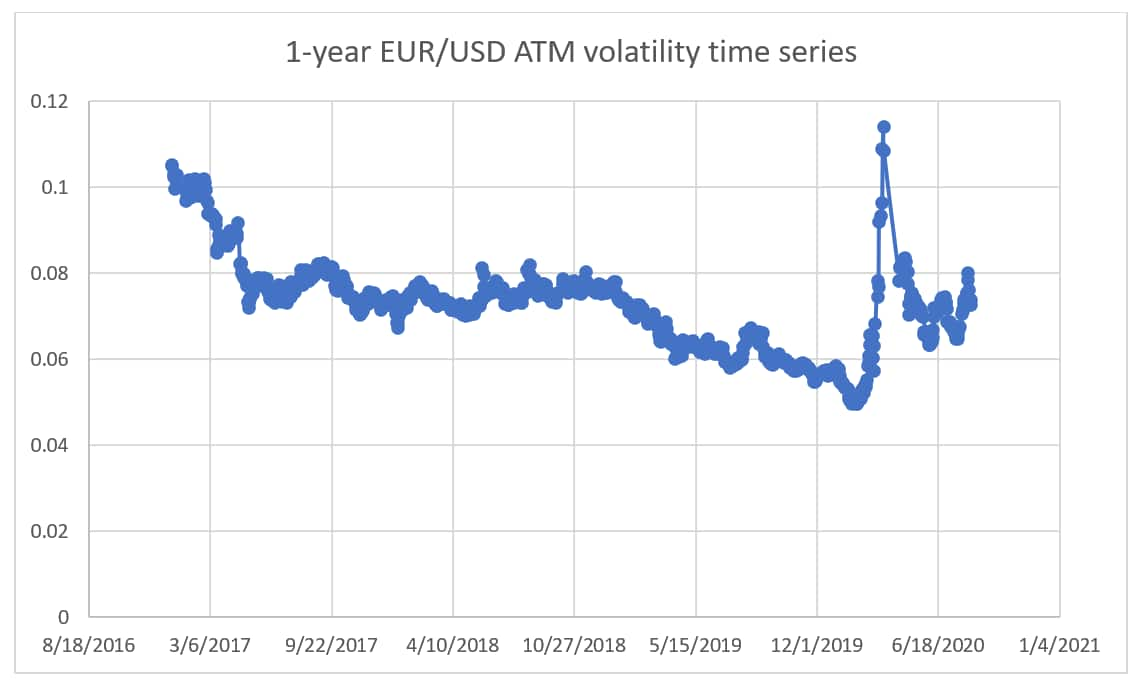
Figure 1. Presence of volatility of volatility.

Modelling volatility of volatility

A volatility risk factor can be included in the simulation in at least two ways:

1. Select a dynamic for the diffusion parameter of the underlying, which leads to a general class of models called stochastic volatility. Some of these models reproduce implied volatility surface and its movements with time. However, they can be difficult to calibrate and the parameters of the dynamic might not be easy to interpret. Vanilla instruments with optionality might also become more difficult to price, usually requiring the need for Fourier theory and some numerical approximations.

2. Select a stochastic process that directly models changes in the observed implied volatility surface, instead of trying to reproduce it by fundamental quantities. This provides an easier framework to jointly simulate all risk factors in the portfolio. It also has the advantage of keeping general analytical methods for pricing intact.

We focus on the second option.

To assess the impact of volatility of volatility on PFE, we look at a set of 1-year European FX call options for various levels of moneyness and compare two use cases, one where the implied volatility surface with the moneyness axis (in relative term F/K, F-K, K/F, K-F) is constant through time (also called sticky delta), and one where the same surface is allowed to change over time. In the base use case, as we simulate risk factors (FX spots or various yield curves) at future dates, each FX option trade will be "travelling" in the domain of the implied volatility surface: toward shorter tenor, and randomly, across the moneyness axis as each scenario holds its own moneyness level.

The sensitivity of price to changes in volatility, the vega, of European options is at its highest at-the-money (ATM) and gets smaller the further it gets from the ATM level. PFE represents the scenarios where each option appreciated. In this case, we use call options, representing the scenarios where the forwards increase considerably, the initial out-of-the-money (OTM) options become closer to the moneyness, and the ATM options are now much more in the money (ITM). This analysis leads us to think that PFE for initial OTM options are more sensitive to the movement of the implied volatility surface and they are going to travel toward a higher vega region in PFE scenarios than their ATM or ITM counterparts.

As our model assumes no bias from the initial volatility surface, we expect the surface to hover around its initial state. For a given tenor, the smile shifts uniformly. For a given level of moneyness, our model implements larger variance to the shorter tenors than the longer tenors. This is in accordance with historical volatility of volatility.

The model also allows the inclusion of correlation to other risk factors. The presence of implied volatility simulation does not, however, modify the marginal distribution of the spots as would a stochastic volatility model like Heston. Therefore, the relationships between implied volatility and other risk factors are left to the correlation parameters. But because PFE is a representation of scenarios with a clear underlying direction (in our example, scenarios with considerably higher moneyness level), including correlation to other risk factors is a clear determinant in the direction of PFE after simulation of volatility. For complete positive correlation to the spot, we expect that scenarios will now also include a shift up in overall volatility.

We face a worst case for credit exposure: spot up, volatility up. But for OTM options, we face an even worse case, where we have travelled to a higher vega region and we also shift the volatility up. This is visible in Figure 2 where PFE is up by 4,000 USD for options that pay 1 million USD. We also note that, in the very short term, it is the ATM options that are most impacted because they have travelled just a little in the implied volatility domain. They remain close to their initial state and the vega is the highest for ATM. However, if the domain of travel increases, OTM options are more affected.

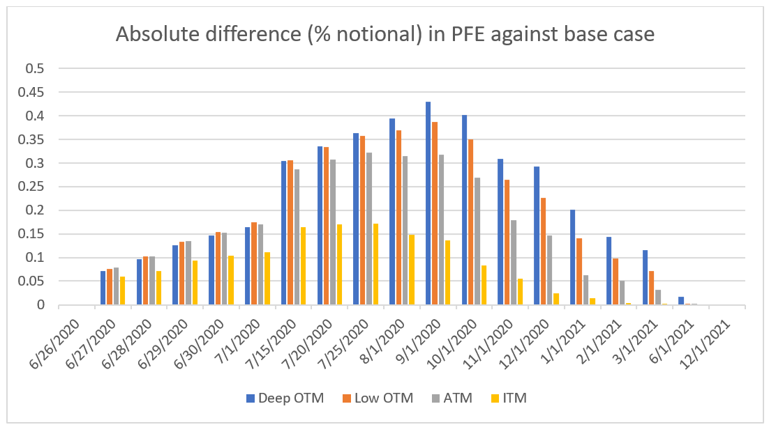
Figure 2. Positive correlation between spot and volatility.

In our analysis, the model for the implied volatility surface is calibrated with the use of time series for a set of ATM options. Using time series from 2017 to 2020, we observe that the correlation between EURUSD spots and EURUSD ATM volatility is negative.

This means the model would predict a compensation of risk and we should see a decreasing PFE as we simulate the surface (see Figure 3a). Compare Figure 3a with Figure 3b to see that if the negative correlation is higher, the impact on PFE is also higher, confirming that the correlation plays an important role in quantifying the impact of simulating implied volatility.

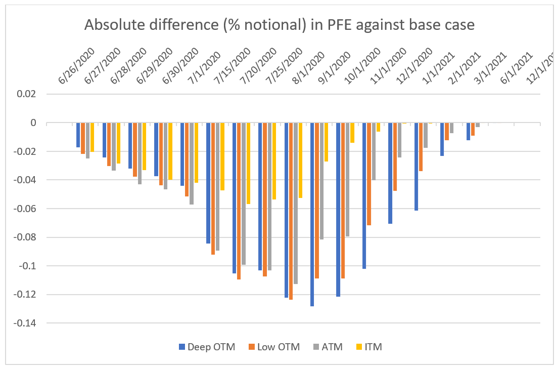
Figure 3a. Historical correlation (-30%) between spots and volatility using the calibration window from 2017 to 2020.

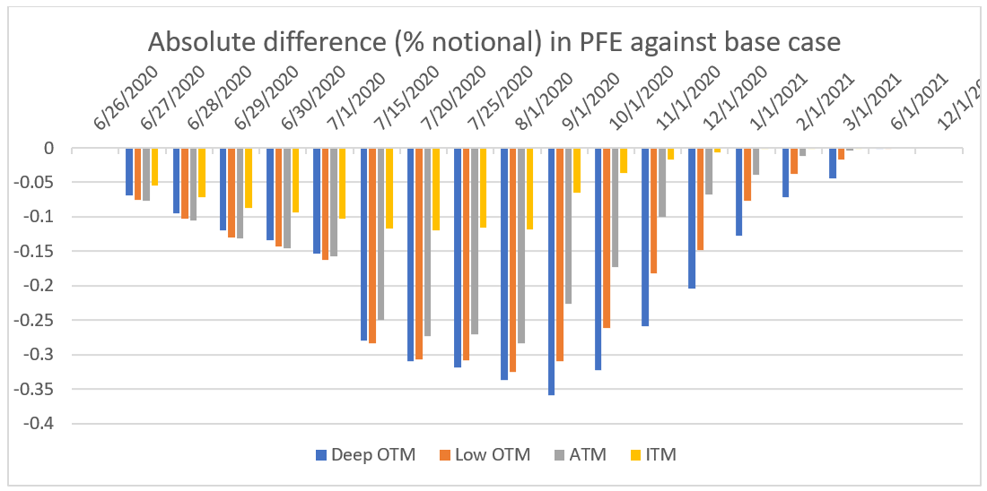
Figure 3b. Perfect negative correlation between spots and volatility.

In a second analysis, we decided to use another calibration window for the volatility model—the first 6 months of 2020—a time where the volatility is observed to be more volatile than usual. As expected, since the volatility of volatility for this model is higher than the previous calibrated model, the impact on PFE is further amplified, as demonstrated when Figure 3b is contrasted with Figure 4.

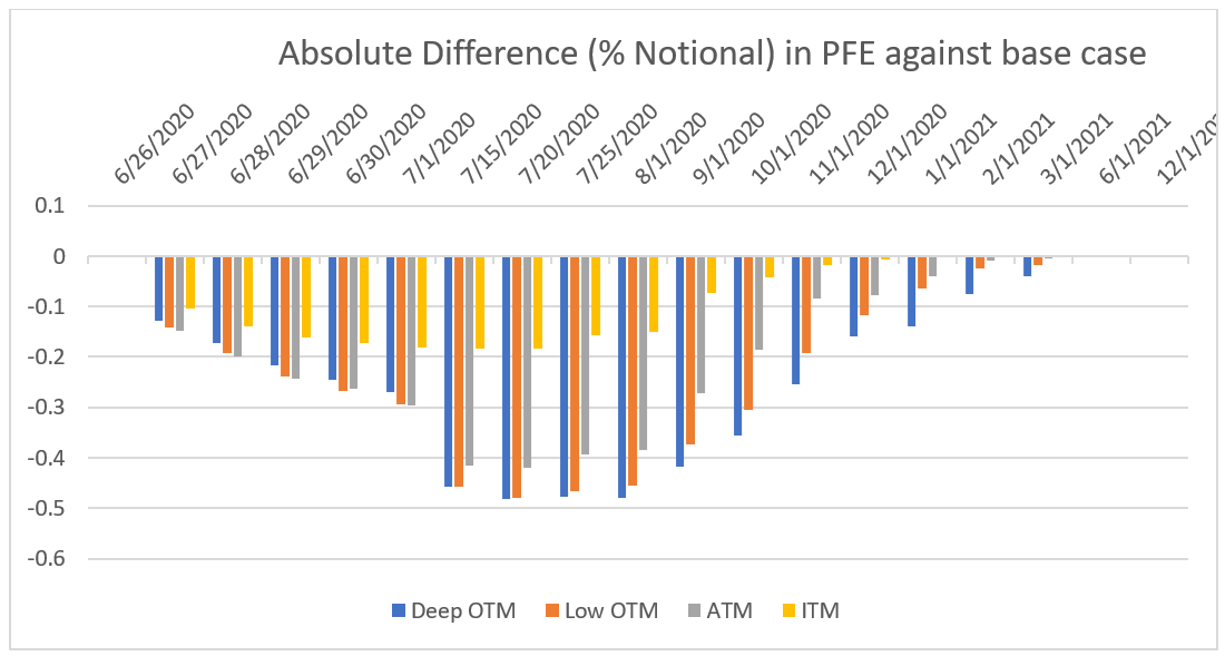
Figure 4. When the volatility model is calibrated to a higher historical volatility period. To compare to Figure 3b perfect negative correlation between spot and volatility is assumed.

For the PFE profile across time, our model suggests that the volatility of the points of the implied volatility surface at longer tenors is lower than the ones at shorter tenors. In the simulation, as we get closer to the expiration of the options, the volatility of volatility tends to get bigger. This means the impact on PFE across time gets bigger. However, these effects get compensated by an extinguishing vega as we get very close to maturity. This leads us to think that the impact of simulating volatility on PFE is at its highest toward the mid-life of instruments, as shown in Figures 2, 3, and 4.

An interpretation of the section of highest impact might be that as the underlying spots progress across time, we progress in the domain of the implied volatility surface on both axes. Depending on how quickly the option reaches low vega region in PFE scenarios that are very close to maturity or deep ITM, the impact on PFE will lower considerably, even if the volatility of volatility gets larger. Thus, the highest impact on the portfolio should be observed sometime before the option expires (time effect of vega) and before OTM options get too deep in the money (moneyness effect of vega).

The future of vega

In this article, we investigated the impact on PFE when volatility of the implied volatility is included in the simulation model. We considered the class of models where the implied volatility surface is directly simulated by a chosen stochastic process calibrated to a volatility time series. Under this model, the marginal distribution of the spot process is unchanged from the base case where volatility is not simulated.

An additional risk this model captures in a bank's portfolio is the right-way or wrong-way risk between the implied volatility and the spot risk factor. The size of the impact on the uncollateralized PFE profile is dictated by:

• Level of the volatility of volatility
• Vega exposure in the portfolio in the PFE scenario at each time step, and
• Correlation between the implied volatility and spot process.

The impact of vega on a collateralized portfolio will be the subject of a future study. Risk managers assessing the quality of their PFE risk engines should carefully consider these three factors and how they impact their uncollateralized exposures.

Potential future exposure (PFE) is a common risk measure used by sell-side banks to manage counterparty credit risk. PFE measures the tail (near worst case) exposure to the counterparty at a future time point. Banks set limits to this tail exposure to cap the risk they face when a counterparty defaults.

Ease the challenge of counterparty credit risk management and capital calculation with S&P Global Market Intelligence

Access a flexible, cloud-based solution that supports counterparty credit risk and regulatory capital requirements.

Keeping up to date with counterparty credit risk regulation is an on-going challenge for banks. After a massive overhaul of the Internal Model Method (IMM) under Basel III, regulation has turned to improving the standardized approach with SA-CCR.

Counterparty Credit Risk from S&P Global helps banks achieve IMM and SA-CCR compliance and is regularly updated in light of regulatory change. Supported by our team of trusted subject matter experts, we help you to reduce the impact, costs and complexity of counterparty credit risk management and capital calculation. Learn more.

[1] St. Clair B. UK budget gives sterling options traders a wild ride. October 6, 2022. https://www.risk.net/derivatives/7954739/uk-budget-gives-sterling-options-traders-a-wild-ride

S&P Global provides industry-leading data, software and technology platforms and managed services to tackle some of the most difficult challenges in financial markets. We help our customers better understand complicated markets, reduce risk, operate more efficiently and comply with financial regulation.

This article was published by S&P Global Market Intelligence and not by S&P Global Ratings, which is a separately managed division of S&P Global.