By Mitsuo Tsumagari

Financial institutions are currently in the process of updating their derivative pricing systems to support Risk Free Rates (RFRs). With the end of IBOR fast approaching (end of 2021) and the amount of work to be done looming over the development teams, some institutions may wonder if approximating RFR payoffs with IBOR payoffs is suitable.

We investigate the quantitative impact for a plain vanilla interest rate swap and European swaption by introducing the three ways of approximating:

1. LEGACY: Use a RFR projection curve in place of the IBOR curve in the legacy IBOR payoff formula

2. PROXY: Use a proxy IBOR projection curve (built to reproduce the value of forward compounded rates) in the legacy IBOR payoff formula

3. OIS: Use RFR projection curve in legacy OIS compounding instruments

Summary:

It is found that a proxy curve can work quite well for approximating the present value of a RFR payoff with a IBOR payoff. However, the approximations deteriorate significantly for forward valuations required for PFE and xVA simulations. Due to the fixing of some of the daily rates contributing to the partially compounded first coupon after valuation, the RFR instruments could not be reproduced by using the legacy IBOR forward rate projection.

An alternative approximation of using an OIS payoff produces better results. However, the OIS legs may incorrectly capture the RFR compounding conventions (look-back, lock-out, backward shift) and may not be available in legacy system for pricing products like notional resetting cross currency swaps, caps and swaptions. In this case, significant approximation errors exist. Given such a legacy system, we found that the maximum future exposure difference from the values with RFR is up to around 200bp by notional in the PFE context and up to around 50 bp in the xVA context. It is good practice to keep monitoring the risk measure errors on PFE/xVA until these banks will fully support the RFR instruments in their risk system.

Set Up:

We consider sample trades of the following product types; interest rate swaps and European swaption. All trades are receiver swaps or receiver swaptions, and the RFRs are daily compounded and backward-shifted. The European swaptions are physically settled. All notionals are set to 1000 and the fixed rates are 1%, and the trade maturities or swap lengths (for swaptions) are 20 years and coupon frequency is semi-annual. The valuation date is February 10 2021. In our setup we assume that banks cannot not use the OIS leg in the swaption case.

Quantitative Results (swaps):

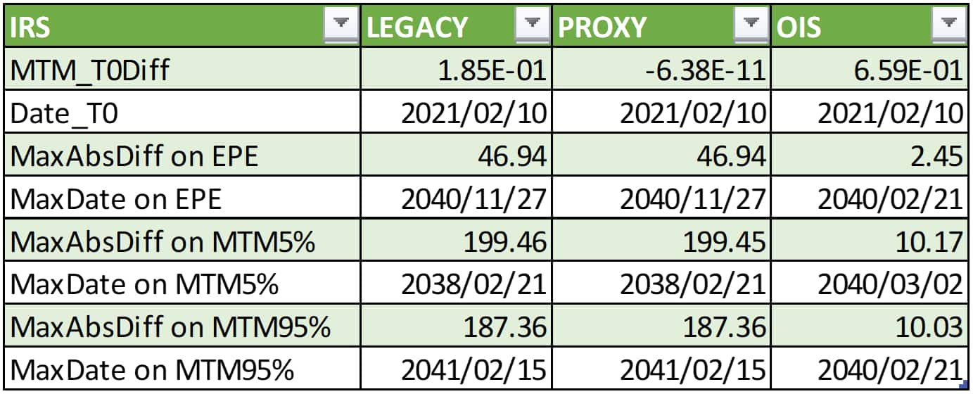
The following table presents the difference from true RFR payoff for three proxy methods. LEGACY method is where the RFR projection curves is used in place of the IBOR projection curve in the IBOR payoff. PROXY approach is where we bootstrap a IBOR projection curve to match with the daily compounded risk-free rates and use that in the IBOR payoff formulas. The OIS approach is where we use the RFR projection curve in existing OIS instruments.

The present value (MTM_T0Diff) matches very well for the PROXY, and less so for the other two methods. This is attributed to the backward shift methodology not being reproduced in those two methods.

The expected positive exposure (EPE) and tails of the distribution at future exposure dates show significantly larger error. We find up to 200 bps error at the worst future exposure date. This quantitative impact would depend on the calibrated model volatility for the yield curve. Our model uses about 20% model volatility and a shifted log-normal model with 100bp shift.

Further insight into the reason for the larger differences at future dates can be seen by plotting the difference in the exposure profiles. In the following figure we plot the future MTM differences at multiple percentile points of the exposure distribution: 1%, 5%, 50%, 95% and 99%, as well as the EPE. The figure contains 6 sub panels. The 3 top panels show the future MTM differences in percentile points over time up to the trade maturity for the LEGACY, PROXY and OIS cases. The 3 bottom panels show the same values in the first 2 years.

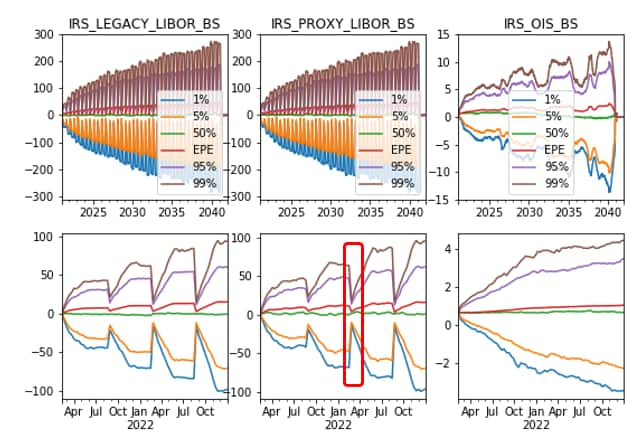
The OIS proxy performs well, with the difference being attributed to the backward shift convention used for RFR compounding. For the LIBOR and PROXY curve approach we see a periodic spike in the error. The periodic frequency corresponds to the semi-annual coupon frequency. We investigate the causes of this error by drilling into the valuation at two consecutive exposure dates 2022/2/15 and 2022/2/25, as highlighted in the red box of the lower middle panel. Note that this IRS trade has the payment dates at 2/20 and 8/20 each year prior to the holiday adjustment and lag.

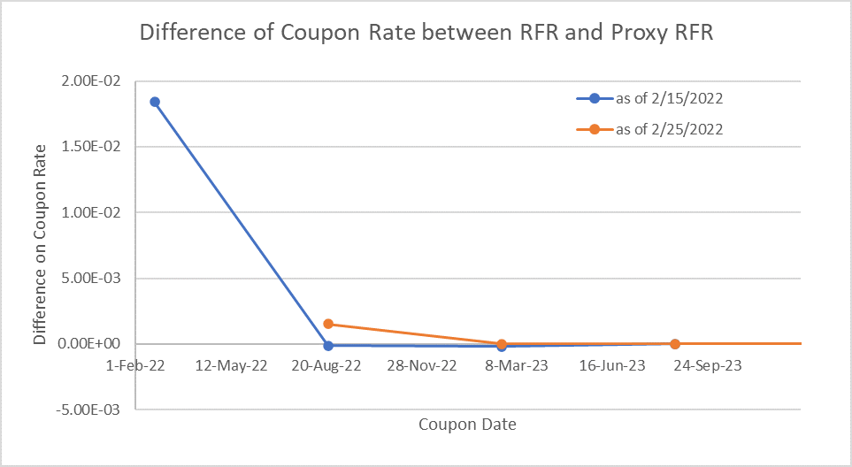
The below figure plots the coupon rate differences (for a single Monte Carlo path) between RFR and PROXY. The blue curve is for February 15 valuation and the orange for Februay 22. Note that a coupon period pays/starts on February 20, part way between these two exposure dates.

The first thing to note is that for the forward starting coupons the projected coupon rates match very well. This is because the payoff formula for geometric compounding reduces to the IBOR payoff formula. However, this is not the case for the partially compounded coupons; the coupon paying February 20 for the blue curve and August 20 for the orange curve. The second thing to note is the error is much larger when the exposure date is near the end of the partially compounded coupon. The exposure date February 15 sits near the end of the coupon period ending February 20, in fact 118 out of the 120 daily compounded rates are already fixed as of this exposure dates. These fixed rates are determined by simulation up to each compounding date. Due to the volatility of rates these can differ significantly from the proxy term Libor calculated at the start of the coupon period. In contrast to this, the exposure date on February 25 sits near the beginning of the coupon period ending August 20. In this case only 5 out of 118 dates in the period are fixed. Hence most of the daily rates are projected with the curve as of the valuation date February 25. The first coupon rate difference causes the large future MTM error. And the first coupon rate difference is caused by projection versus simulation of the RFR rates to their fixing dates.

Using the OIS leg, the fixing of the daily compounded rates is accurately captured. This fact explains why the maximum MTM differences for OIS are much smaller than the other two cases, i.e. LEGACY and PROXY. The relatively small difference with the OIS leg is caused by the RFR averaging type difference.

Quantitative Results (swaptions):

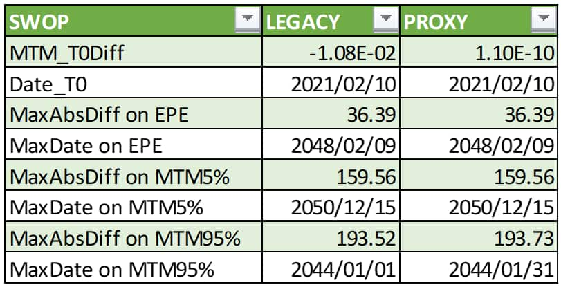
We repeat the same analysis for swaption trades, i.e. European swaptions with 10 years option expiry by 20 years underlying swap. However, we don't include the OIS proxy as it is assumed that OIS swaptions are not available in the legacy library.

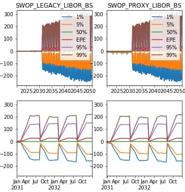
Similar results are found as in the swap case. Present value is well approximated by the proxy curve, however forward valuations show significant errors.

The below figure plots the difference in the exposure profile for the swaption. Before exercise the proxies behave quite well, but after exercise we observe the same periodic spike in error. This error is attributed to the error in the partially compounded coupon rates of the swap that the swaption has exercised into.

Recap:

We have seen that it is successful to introduce the proxy RFR curve for computing the present value for swaps and swaptions. However, the proxy behaves poorly when used for future exposure calculations. Banks with the OIS swap legs can approximate PFE with the RFR swaps very well. However, if the OIS leg is not available for swaptions they have to use the legacy IBOR based swaptions instead, and in this case significant errors are found. Those banks should pay attention on the large PFE errors (200 bps in our example). In the xVA context, the calculation is based on the EPE profile. The EPE differences from RFR with the legacy leg are around 50 bp and 40 bp, respectively, in both swaps and swaptions. It is good practice to keep monitoring the pricing errors on PFE/xVA until these banks will fully support the RFR instruments in their risk system.